Solar PV systems and trees methods
Methodology[edit | edit source]
In this paper, a method will be introduced to simulate the shadow pattern of different trees. Trees will be placed at different locations on south side of the house. The minimum distance will be determined for planting trees so that no shade will fall over the panels between 10 am and 2 pm.
The methodology of this paper is as follows
- Choosing a pilot region for the case study.
- Study of the trees that are found in the chosen region.
- Choosing sample trees for the case studies.
- Calculating the tree growth and the growth of the tree crown by using the mathematical expressions.
- Choosing a pilot location and orienting the roof (gable, where the solar PV array will be installed) of the house facing south - assuming northern hemisphere.
- Locating the chosen trees on the south side of the house.
- Simulating the pattern of the shadow.
- Finding the optimal distances for different type of trees so that there will be no shade on the PV system as the tree grows - while keeping them as close to the house as possible.
Choosing the Region[edit | edit source]
Midwest United States is the chosen region for this study and the pilot location will be Michigan. The most common trees were found after a comprehensive literature review about trees. These trees and their percentages are given in table below.[1]
| Rank | Common Name | Percent | Cumulative Percent |
|---|---|---|---|
| 1 | Silver Maple | 22.65 | 22.65 |
| 2 | Sugar Maple | 8.05 | 30.70 |
| 3 | Norway Maple | 7.02 | 37.71 |
| 4 | Green Ash | 6.71 | 44.42 |
| 5 | American Elm | 4.59 | 49.01 |
| 6 | Red Maple | 4.52 | 53.52 |
| 7 | White Ash | 3.44 | 56.97 |
| 8 | Honeylocust | 3.25 | 60.22 |
| 9 | Siberian Elm | 2.98 | 63.20 |
| 10 | Hackberry | 2.57 | 65.77 |
| 11 | Crabapple | 2.09 | 67.86 |
| 12 | Pin Oak | 1.92 | 69.78 |
| 13 | American Sycamore | 1.75 | 71.53 |
| 14 | Little-leaf Linden | 1.68 | 73.21 |
| 15 | Northern Red Oak | 1.37 | 74.58 |
| 16 | Mulberry | 1.30 | 75.88 |
| 17 | Eastern Cottonwood | 1.15 | 77.03 |
| 18 | American Basswood | 1.12 | 78.16 |
| 19 | Eastern White Pine | 0.99 | 79.15 |
| 20 | Northern Catalpa | 0.99 | 80.14 |
| 21 | Colorado Blue Spruce | 0.93 | 81.07 |
| 22 | Sweetgum | 0.92 | 81.99 |
| 23 | Tulip Tree | 0.92 | 82.91 |
| 24 | Boxelder | 0.92 | 83.83 |
| 25 | Pear | 0.91 | 84.74 |
Study of Tree Types[edit | edit source]
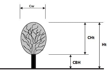
The amount of shadow from a tree depends on the following;
- Tree height
- Height of the tree crown
- Width of the tree crown
- Type of the tree crown, conical, rounded or oval
Height of the tree and crown and the crown width are function of time and they change with respect to year. Change in these parameters essentially change the size of the shadow. So, it is important to know the mathematical expressions of these time dependent parameters. Sugar Maple and White Pine are two tree types that will be used in this paper to demonstrate the method we use. Mathematical expressions of the these trees are given below. Unfortunately, the equations to predict the dimensions are available only for certain trees. Silver Maple, Sugar Maple, Norway Maple, Green Ash, Red Maple, Hackberry, Little-leaf Linden, American Basswoood and White Pine are the trees with available equation and coefficients. For trees with no available equation to predict their dimensions, average height and crown width at maturity can be used for the simulations.
Approximated Diameter at Breast Height (DBH) for Sugar Maple and White Pine[edit | edit source]
| Species | B0 | B1 | B2 |
|---|---|---|---|
| Sugar Maple | 30.49 | -0.0308 | 1.836 |
| White Pine | 43.859 | -0.0181 | 1.503 |
Approximated Tree Height(Ht) for Sugar Maple and White Pine[edit | edit source]
| Species | B0 | B1 | B2 |
|---|---|---|---|
| Sugar Maple | 4 | 7.5 | 0.6 |
| White Pine | 5.73 | 2.615 | 1.033 |
Approximated Crown Width(Cw) for Sugar Maple and White Pine[edit | edit source]
| Species | B0 | B1 | B2 |
|---|---|---|---|
| Sugar Maple | -0.543 | 4.691 | 0.688 |
| White Pine | 1.634 | 3.628 | 0.723 |
Approximated Crown Height(CHt) for Sugar Maple and White Pine[edit | edit source]
| Species | B0 | B1 | B2 |
|---|---|---|---|
| Sugar Maple | -3.98 | 8.873 | 0.306 |
| White Pine | 3.087 | 0.468 | 1 |
Predicting the Shadow Patterns[edit | edit source]
Sample trees will be located on south since the PV arrays are placed facing south. Using the mathematical expressions, trees will be modeled. A one story house will be modeled as it is shown in the Figure. Shadow prediction will be made by using Heliodon Model [1]. There is a demo version of the Heliodon software is available online which can be utilized or real Heliodon structure can be built for shadow pattern prediction. There is also Google Sketchup 8 available online at no cost and it is able to simulate the shadow patterns of the objects. 3D Warehouse is a website where most of the 3D objects can be found and downloaded for free as well.
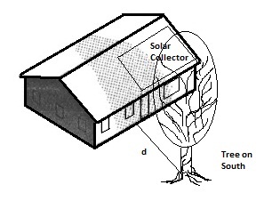
Google Sketchup 8 Simulations[edit | edit source]
For shadow simulations, first important step is to choose the geographic location. The area of the shadow and the path that shadow will follow depends on the location. After opening the Google Sketchup, the geographic location can be selected under File->geo location->add location.
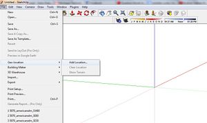
After clicking on add location, the google map will open up and from the map, any location can easily be chosen. User needs to enter his/her password for the gmail account.
3D models can be downloaded from 3D warehouse within Google Sketchup. To do so, click on, file->3D warehouse->Get models, see Fig 4.

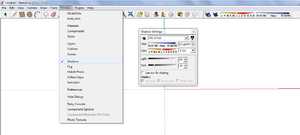
Components and models can be rescaled to adjust their height and width. To scale any component, just click on the component and press "S" on the keyboard, or go to tools and choose scale. Then the component can be rescaled by stretching it from the expansion points using mouse. Solar panels are placed on rooftop facing south. In this simulations, trees will be placed on south side of the house. It is important to note that the Green Line on Google Sketchup points North. Once the components are found and imported on Google Sketchup, the next step will be choosing the time of the year and the time of the day. Choosing the time zone is also recommended. All these setting can be done under the shadow setting tab which can be opened up by clicking window->shadows, see Fig 5.
Finding the Optimal Distance for Tree Planting[edit | edit source]
Trees will be placed at geometrically defined lines, namely, W, SW30, SW60, 90, SE60, SE30 and E. See Fig 6. The distance between the tree and the house will be increased by dragging the tree far away from the house. The optimu point will the the spot will the place where the tree cast no shade over the PV panels between 10 am and 2 pm. The distance between the tree and the house can be measured by using tape measure tool.
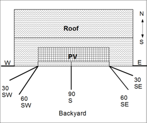
Fig 7 shows the screen shot of the simulation made on Google Sketchup 8 with components downloaded from 3D Warehouse.


