User:Amitd/Sandbox

Deformity Correction Of Lower Limb Bones[edit | edit source]

The materials in this course encompass the cognitive learning and the psychomotor skills necessary to become a certified orthopedic surgeon skilled in complex bone deformity planning. Note that this does not cover the complete set of knowledge-based information for complex bone deformity planning, however, it helps prepare you for both the core skill and the supplemental skills required. They are listed in the order in which they should be learned, with a focus on mastering the fundamentals first, as some of the later skills build upon techniques learned in earlier skills.

1. Line Diagram

To understand complex bone deformities, it is important to first understand and establish the parameters and limits of normal alignment.
The exact anatomy of the femur, tibia, hip, knee, and ankle is of great importance to the clinician when examining the lower limb and to the surgeon when operating on the bones and joints.
To better understand alignment and joint orientation, the complex three-dimensional shapes of bones and joints can be simplified to basic line drawings (Fig. 1a)

For purposes of reference, these line drawings should refer to either the frontal, sagittal, or transverse anatomic planes.
The two ways to generate a line (Fig. 1b) in space are either a) to connect two points or b) to draw a line through one point at a specific angle to another line.
All the lines that we use for planning and for drawing schematics of the bones and joints are generated using one of these two methods.

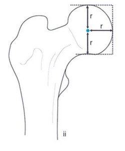
2. Joint Center Points

The joint center points of hip, knee and ankle joints are defined in the frontal plane
Fig. 2a
For the hip joint or the proximal femur region, the joint center point is the center of the circular femoral head (Fig. 2a)
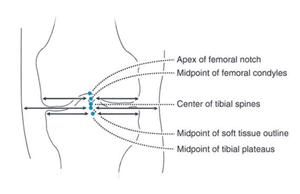
Fig. 2b
For the knee joint or the distal femur region, the joint center point is the apex of the femoral notch (Fig. 2b)
Fig. 2c
For the knee joint or the proximal tibia region, the joint center point is the center of the tibial spines (Fig. 2b)
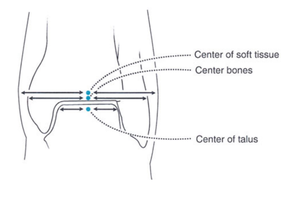
For the ankle joint or the distal tibia region, the joint center point is the center of the talus or plafond (Fig. 2c)

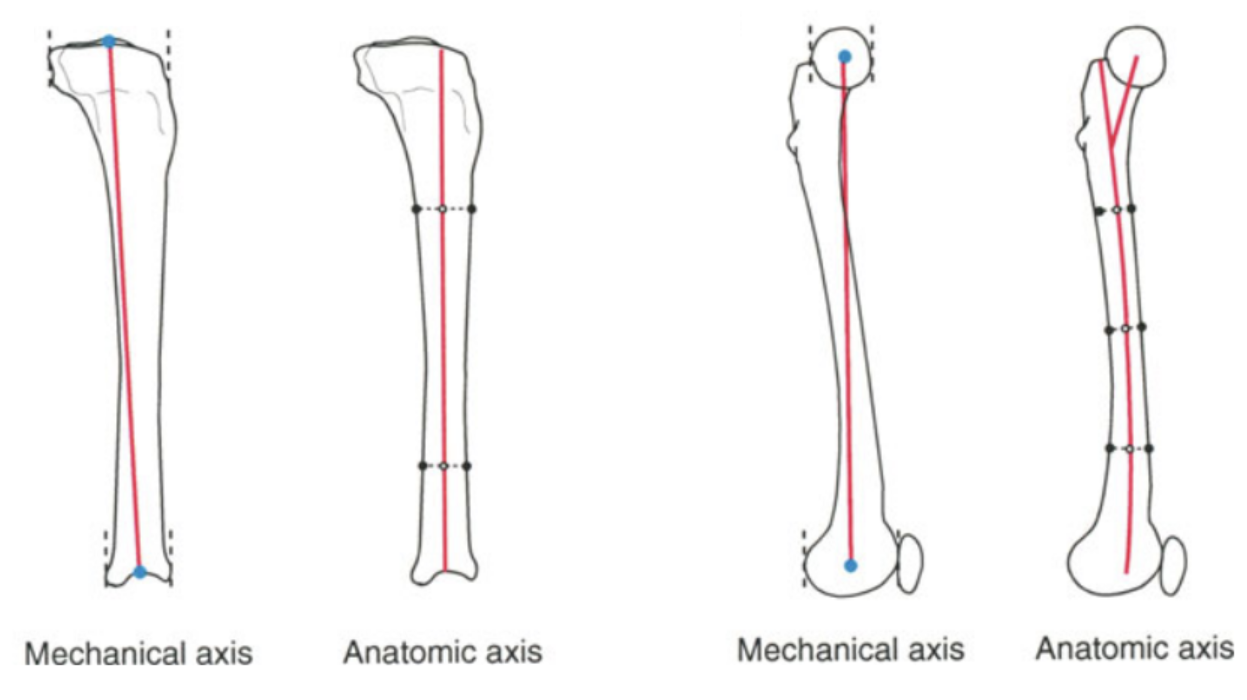
3. Axes of the long bones - Mechanical and Anatomical

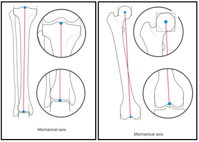
Fig. 3a
The mechanical axis of a long bone is a straight line connecting the joint center points of the proximal and distal joint regions, whether in the frontal or sagittal plane (Fig. 3a).
The anatomic axis of a bone is the mid-diaphyseal line (Fig. 3b). The anatomic axis line may be straight in the frontal plane but curved in the sagittal plane, as in the femur.
Fig. 3b
In the tibia, the frontal plane mechanical and anatomic axes are parallel and only a few millimeters apart. Therefore, the tibial anatomic-mechanical angle (AMA) is 0° (Fig. 3c)
In the femur, the mechanical and anatomic axes are different and converge distally. The normal femoral AMA is 7±2° (Fig. 3c)

4. Joint Orientation Lines/ Joint Lines

Joint Orientation Line or Joint Line is a line representing the orientation of the joint in a frontal or sagittal plane
The orientation of the hip joint in the frontal plane can be described by ‘Proximal Femoral Joint line’ as a line joining the tip of greater trochanter and the femoral head center (Fig. 4a)

The orientation of the hip joint in the frontal plane can also be alternatively described by ‘Femoral Neck Line’ as a line joining the femoral head center and mid-diaphyseal width of the femoral neck (Fig. 4b)

The frontal plane knee joint line of distal femur or ‘Distal Femoral Joint Line’ is drawn as a line tangential to the most distal point on the convexity of each of the two femoral condyles (Fig. 4c)

The frontal plane knee joint line of proximal tibia or ‘Proximal Tibial Joint Line’ is drawn across the flat or concave aspect of the subchondral line of the two tibial plateaus (Fig. 4d)

In the sagittal plane, Proximal Tibial Joint Line is drawn along the flat subchondral line of the tibial plateaus (Fig. 4e)

In the sagittal plane, Distal Femoral Joint Line be drawn as a straight line connecting the two points where the femoral condyles meet the metaphysis of the femur (Fig. 4f)

The frontal plane ankle joint line or ‘Distal Tibial Joint Line’ is drawn across the flat subchondral line of the tibial plafond in either the distal tibial subchondral line or for the subchondral line of the dome of the talus (Fig. 4g)

In the sagittal plane, Distal Tibial Joint Line is drawn from the distal tip of the posterior lip to the distal tip of the anterior lip of the tibia (Fig. 4h)

5. Joint Orientation Angles/Angular parameters of the long bones

The joint lines in the frontal and sagittal planes have a characteristic or well-defined orientation to the mechanical and anatomic axes. This is defined as Joint Orientation Angles
The name of each angle specifies whether it is measured relative to a mechanical (m) or an anatomic (a) axis. The angle may be measured medial (M), lateral (L), anterior (A), or posterior (P) to the axis line. The angle may refer to the proximal (P) or distal (D) joint orientation angle of a bone (femur [F] or tibia [T])
The mechanical lateral distal femoral angle (mLDFA) is the lateral angle formed between the mechanical axis line of the femur and the knee joint line of the femur in the frontal plane.
The anatomic lateral distal femoral angle (aLDFA) is the lateral angle formed between the anatomical axis line of the femur and the knee joint line of the femur in the frontal plane.
The lateral proximal femoral angle (LPFA) is the lateral angle formed between the mechanical axis line of the femur and the proximal joint line of the femur in the frontal plane
The medial proximal femoral angle (MPFA) is the medial angle formed between the anatomical axis line of the femur and the proximal joint line of the femur in the frontal plane.
The medial neck shaft angle (MNSA) is the medial angle formed between the anatomical axis line of the proximal femur and the neck axis of the femur in the frontal plane.
The posterior distal femoral angle (PDFA) is the posterior angle formed between the anatomical axis line of the distal femur and the distal joint line of the femur in the sagittal plane.
The medial proximal tibial angle (MPTA) is the medial angle formed between the mechanical axis or anatomic axis line of the tibia and the knee joint line of the tibia in the frontal plane.
The lateral distal tibial angle (LDTA) is the lateral angle formed between the mechanical axis or anatomic axis line of the tibia and the distal joint line of the tibia in the frontal plane.
The posterior proximal tibial angle (PPTA) is the posterior angle between the anatomic axis of the tibia and the proximal joint line of the tibia in the sagittal plane

The anterior distal tibial angle (ADTA) is the anterior angle between the anatomic axis of the tibia and the distal joint line of the tibia in the sagittal plane.

The joint line convergence angle (JLCA) is the angle formed between the femoral distal joint line and tibial proximal joint line in the frontal plane
The schematic drawings of the nomenclature of the mechanical and anatomical frontal and sagittal joint angles and their normal ranges are described in the below figures (Fig. 5a, 5b and 5c)

6. Mechanical Axis Deviation (MAD) and Hip-Knee-Ankle angle (HKA)

The mechanical axis of the leg is different from the mechanical axis of femur and tibia. It is defined as line drawn from femoral head center to the ankle center
The distance between the leg mechanical axis line and the center of the knee in the frontal plane is called the Mechanical Axis Deviation (MAD). The normal range of MAD is 8+/-7 mm medially (Fig. 6a)
The MAD is described as either medial or lateral. Medial and lateral MADs are also referred to as varus or valgus malalignments, respectively (Fig. 6b)
The HKA angle is the medial angle between the mechanical axis line of femur and mechanical axis line of tibia in the frontal plane.
The normal range of HKA is 180 +/- 3°. If HKA < 177°, leg is known as to be in varus malalignment and if HKA > 183°, leg is in valgus malalignment (Fig. 6b)

7. Malalignment and Malorientation - Source of Deformity

Malalignment : refers to loss of collinearity of the hip, knee & ankle in the frontal plane ( MAD exceeds normal range)
Malalignment Test (MAT): Draw mechanical axes and knee joint lines. Measure the mechanical angular parameters - mLDFA and MPTA
MAT 1: If MAD exceeds normal range and (MPTA < 85° (tibial varus deformity) or mLDFA > 90° (femoral varus deformity) or both (tibia and femur varus deformity)), it is a varus malalignment of the limb (Fig. 7a)
MAT 2: If MAD exceeds normal range and (MPTA > 90° (tibial valgus deformity) or mLDFA < 85° (femoral valgus deformity) or both (tibia and femur valgus deformity)), it is a valgus malalignment of the limb (Fig. 7b)
MAT 3: If MAD exceeds normal range and varus JLCA > 2°, it is varus malalignment due to deformity in knee joint. If MAD exceeds normal range and valgus JLCA > 2°, it is valgus malalignment due to deformity in knee joint (Fig. 7c)
Malorientation Test (MOT): Draw mechanical axes and draw proximal femur joint lines and distal tibia joint lines. Measure the LPFA and LDTA angles. If they are not in normal range, there is malorientation in the hip joint or ankle joint or both (Fig. 7d).
Malalignment (MAT) is Malorientation (MOT) for the knee joints.
Malorientation of the ankle or hip joints usually leads to minimal or no MAD because the deformity apex is at or near the ends of the mechanical axis of the lower limb (refer Fig. 7d)

8. Mechanical and Anatomical Axis Planning - Frontal plane

When there is Malalignment or Malorientation in femur or tibia bones, the bone with deformity can be divided into proximal and distal bone segments. The proximal and distal bone segments have their own proximal mechanical axis (PMA) or proximal anatomical axis (PAA) line and distal mechanical axis (DMA) or distal anatomical axis (DAA) line respectively (Fig. 8a)
The point at which the proximal and distal axis lines intersect is known as the Center of rotation of angulation (CORA). (Fig. 8b)
The PMA or DMA lines can be drawn from respective joint centers taking normal values of joint orientation angle as reference (Fig. 8b).
The acute angle between the two axis lines (PMA and DMA) or (PAA and DAA) is the ‘Magnitude (Mag) of correction’ required to correct the deformity in the bone (Fig. 8b). This is also called the ‘Correction angle’.
The PAA and DAA lines can be drawn taking mid-diaphyseal lines in the proximal shaft or the distal shaft bone segment respectively or drawing axis lines taking normal values of anatomical angles from the joint lines (Fig. 8c).
The bone deformity can be corrected by performing an osteotomy (bone cut) near CORA calculated from the deformity planning in frontal plane and rotating the distal bone segment by ‘Correction angle’ about an imaginary Angulation Correction Axis (ACA) which may or may not pass through CORA (Fig. 8b). Many times ACA is also referred to as ‘hinge’ or ‘pivot’ about which the resected bone segment rotates.
There are three rules of Osteotomy which summarises the correction of a deformed bone.
Osteotomy Rule 1: If the ACA passes through the CORA (ACA-CORA) , and the osteotomy line or level also passes through CORA, then the resected bone segment will only angulate with respect to the other bone segment without any translation or displacement at the osteotomy level. The proximal axis and distal axis lines will become collinear and parallel if the magnitude of angulation is equal to the ‘Correction angle’ (Fig. 8d)

Osteotomy Rule 2: If the ACA passes through the CORA (ACA-CORA), but the osteotomy line or level is above or below the CORA, then the resected bone segment will angulate and also translate with respect to the other bone segment at the osteotomy level. The proximal axis and distal axis lines will become collinear and parallel if the magnitude of angulation is equal to ‘Correction angle’ (Fig. 8e)
Osteotomy Rule 3: If the ACA does not pass through the CORA, and the osteotomy line or level is at the ACA, then the resected bone segment will only angulate with respect to the other bone segment at the osteotomy level. The proximal axis and distal axis lines will become only parallel and not collinear, if the magnitude of angulation is equal to ‘Correction angle’. The resulting bone correction will induce a ‘translation deformity’ between the two bone segments. (Fig. 8f)
The osteotomy can be performed by doing an opening wedge osteotomy, a closing wedge osteotomy or a neutral wedge osteotomy
Opening wedge osteotomy: In this kind of osteotomy, the ACA-CORA is at the convex cortex of the bone and also called as the opening wedge point. The osteotomy line or level passes through the opening wedge point. The convex cortex remains in contact whereas the concave side is fully distracted or opened by an angle equal to the correction angle in angular terms and a length ‘L’ at the most concave side. The bone is lengthened by the same length ‘L’ (Fig. 8g)
Closing wedge osteotomy: In this kind of osteotomy, the ACA-CORA is at the concave cortex of the bone and also called as the closing wedge point. The osteotomy line or level passes through the closing wedge point. The concave cortex remains in contact whereas at the convex side, the bone wedge is removed by an angle equal to the correction angle in angular terms and a length ‘L’ at the most convex side. The bone is shortened by the same length ‘L’. The two bone segments come in full bone-to-bone contact at the end of correction (Fig. 8h)
Neutral wedge osteotomy: In this kind of osteotomy, the ACA-CORA is in between the concave and convex cortex of the bone and also called as the neutral wedge point. The osteotomy line or level passes through the neutral wedge point. There is partial opening wedge at the concave cortex and partial closing wedge at the convex cortex. The bone wedge is removed by an angle equal to the correction angle in angular terms and a length ‘L/2’ at the most convex side compared to the closing wedge osteotomy length ‘L’. The bone is lengthened by the length ‘L/2’ compared to the opening wedge length ‘L’. All parts of the bone convex to the neutral wedge point come in full bone-to-bone contact whereas in the concave part reactive to the neutral wedge there is a gap between the bone segments (Fig. 8i)
The bone angulation deformity can be seen in either the frontal plane (visible on AP x-rays) or sagittal plane (visible on LAT x-rays) or both.
These angulation deformities can be at one level or location in the bone referred to as ‘Uniapical deformity’ or it can be at multiple locations also referred to as ‘Multiapical deformity’ (Fig. 8j)

9. Mechanical and Anatomical Axis Planning - Sagittal plane

When there is Malalignment or Malorientation in femur or tibia bones in sagittal plane, the proximal and distal bone segments have their own proximal mechanical axis (PMA) or proximal anatomical axis (PAA) line and distal mechanical axis (DMA) or distal anatomical axis (DAA) line respectively in the sagittal plane (Fig. 9a)
Draw anatomical axis of proximal shaft and anatomical axis of distal shaft. The point of intersection of the axes is CORA and the magnitude of acute angle formed is the magnitude of correction angulation required (Fig. 9b)
Draw anatomical reference line from proximal joint line of tibia at (1/5th width of condyle) and anatomical axis of the shaft or anatomical reference line at normal ADTA angle of 80 from the distal joint line. The point of intersection of the axes is CORA and the magnitude of acute angle formed is the magnitude of correction angulation required (Fig. 9c)

10. Oblique Plane Deformity

Angular deformity in long bones can occur in any plane. Deformities in which angulation is seen on both AP and LAT x-rays are actually uniapical deformities in an oblique plane. They are also known as ‘Oblique plane deformities’(Fig. 10a)

To plan an oblique plane deformity case, two important parameters are required. One is the ‘angle of the oblique plane’ itself w.r.t the AP and LAT direction. Second is the ‘magnitude of angulation deformity’ which the bone has in this oblique plane. Both these parameters can be calculated by a simple method called ‘Graphical method’ explained as follows.
Step 1: First draw a graph with orthogonal x-axis and y-axis. The x-axis represents the frontal plane (AP view) and the y-axis represents the sagittal plane (LAT view). It is drawn in such an orientation by imagining that you are viewing your own foot from the top. The plane of the graph represents the Transverse plane of the body
Step 2: The positive y-axis represents the anterior (A) side while the negative y-axis represents the posterior (P) side for both right and left leg. For the left leg, the positive x-axis represents the medial (M) side while the negative x-axis represents the lateral (L) side. For the right leg, the negative x-axis represents the medial (M) side while the positive x-axis represents the lateral (L) side. Label the graph appropriately (Fig. 10b)
Step 3: Mark the magnitude of angulation in the bone in AP and LAT view on the graph taking 1 mm = 1° as the scale. For the right leg, if AP angulation is varus (vr), mark the angular correction angle on the positive x-axis and if it is valgus (vl), it is negative x-axis. For the right leg, if LAT angulation is procurvatum (pr), mark the angular correction angle on the positive y-axis and if it is recurvatum (re), it is negative y-axis (Fig. 10c)
Step 4: Draw a line from origin (0,0) to magnitude of (ap, lat) angulation value (Fig. 10d)
Step 5: Measure the length of this newly drawn oblique line, then that value will become the ‘magnitude of angulation’ in the oblique plane. Measure the angle between the oblique line and the x-axis (lateral), then that value will become the ‘oblique plane angle’ from the front (AP) view (Fig. 10e). Now the deformity can be planned in this oblique plane like planning done in normal uniapical deformity in AP or LAT view. The ‘magnitude of angulation’ is the correction angle for osteotomy in this oblique plane.

11. External fixation devices - Rail Fixator

The most common rail fixators consist of three parts namely clamp, rail rod and the schanz screws (Fig. 11a)

The clamp has a dovetail profile which slides onto the rail rod and is tightened onto the rail rod by tightening the holding screws on the clamp (Fig. 11a)
There is a type of rail external fixator called a monolateral fixator which is a single unit with proximal and distal clamps attached together by an hinge (for angulation) and linear actuator (for compression or distraction of two bone segments) (Fig. 11b)

The hinge of the monolateral fixator should always lie on the angle bisector of the planned proximal and distal axis on the bone (Fig. 11c)
The angulation of the fixator should be of the same angle as the magnitude of angulation of the bone (Fig. 11c)

When the correction of bone happens taking hinge of rail fixator as the ACA and it passes through the angle bisector line of the planned axis, then the resultant proximal and distal axis becomes parallel and vertical Lengthening (‘SL’) of distal segment occurs w.r.t proximal bone segment (Fig. 11c)
When the correction of bone happens taking hinge of rail fixator as the ACA and it passes above or below the angle bisector line of the planned axis, then the resultant proximal and distal axis becomes parallel but horizontal Translation (‘ST’) of distal segment occurs w.r.t proximal bone segment (Fig. 11d)